Bernstein-Vazirani Algorithm
The Bernstein–Vazirani algorithm was invented by Ethan Bernstein and Umesh Vazirani in 1997. The Bernstein–Vazirani problem is defined as follows:
Problem Definition
Given a function \(f∶\left\{0,1\right\}^n\mapsto\left\{0,1\right\}\), with the oracle function \(f(x)=a\cdot x\), where a is a constant vector of \(\left\{ 0,1 \right\}^n\), and \(a\cdot x\) is a scalar product of a and`x`. The goal of the oracle is to find the hidden bit string a.
A classical solution to this problem requires n steps. We can retrieve the hidden string \(a(a_0 a_1 a_2\ldots a_{n-1} )\) by querying the oracle with a value of x, such that each query returns one of the bits in the hidden string. For example:
After querying all the bits, we can stitch the results and obtain the hidden string \((a_0 a_1 a_2 a_3)\). There are a few ways to solve this problem on a quantum computer, and we can get the answer in one step. The block diagram [15] for the solution to the Bernstein-Vazirani oracle is given below.
We can implement the oracle function as a set of CNOT gates, with the ancilla qubit as the target and the data register qubits corresponding to the bit value of the hidden string a as the control qubits. The following figure [16] illustrates this for a hidden string \(10 =1010b\).
For a detailed step-by-step math of this algorithm, see [10]. The source code for this oracle is outlined in the following sections.
Note
Be sure to use your API token and your account name.
Step 1. Import the required modules and obtain the backend
import QuantumRingsLib
from QuantumRingsLib import QuantumRegister, AncillaRegister, ClassicalRegister, QuantumCircuit
from QuantumRingsLib import QuantumRingsProvider
from QuantumRingsLib import job_monitor
from QuantumRingsLib import JobStatus
from matplotlib import pyplot as plt
import numpy as np

provider = QuantumRingsProvider(token =<YOUR_TOKEN_HERE>, name=<YOUR_ACCOUNT_NAME_HERE>)
backend = provider.get_backend("scarlet_quantum_rings")
shots = 100

provider.active_account()
Step 2. Define the core methods
def bv_func (qc, hiddenstring):

    # set the ancilla qubit to state |1>
    qc.x(qc.num_qubits-1)

    # Set all qubits to a superposition state.
    for i in range (qc.num_qubits):
        qc.h(i)

    qc.barrier()

    # implement the hidden string - the oracle function
    for i in range (qc.num_qubits - 1):
        if ( 0!= ( hiddenstring & (1 << i))):
            qc.cx(i, qc.num_qubits-1)

    qc.barrier()

    # Apply H gates one more time
    for i in range (qc.num_qubits-1):
        qc.h(i)

    qc.barrier()

    # finally measure
    for i in range(qc.num_qubits - 1):
        qc.measure(i,i)

    return

def plot_histogram (counts, title=""):
    """
    Plots the histogram of the counts

    Args:

        counts (dict):
            The dictionary containing the counts of states

        titles (str):
            A title for the graph.

    Returns:
        None

    """
    fig, ax = plt.subplots(figsize =(10, 7))
    plt.xlabel("States")
    plt.ylabel("Counts")
    mylist = [key for key, val in counts.items() for _ in range(val)]

    unique, inverse = np.unique(mylist, return_inverse=True)
    bin_counts = np.bincount(inverse)

    plt.bar(unique, bin_counts)

    maxFreq = max(counts.values())
    plt.ylim(ymax=np.ceil(maxFreq / 10) * 10 if maxFreq % 10 else maxFreq + 10)
    # Show plot
    plt.title(title)
    plt.show()
    return
Step 3. Execute the algorithm and plot the results
# obtain the hidden string from the user
hiddenstring = int(input("Enter the hidden string as a binary value: "), 2)

#determine the number of qubits required to represent the hidden string
numberofqubits = hiddenstring.bit_length()

print(hiddenstring, numberofqubits)

# add a qubit for the ancilla register
numberofqubits += 1

q = QuantumRegister(numberofqubits , 'q')
c = ClassicalRegister(numberofqubits , 'c')
qc = QuantumCircuit(q, c)

bv_func(qc, hiddenstring)

job = backend.run(qc, shots=shots)
job_monitor(job)
result = job.result()
counts = result.get_counts()

plot_histogram(counts,"")
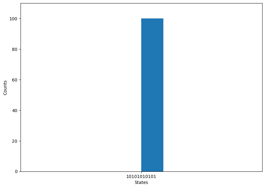
An example histogram is shown below for the hidden string \(10101010101\).

Bernstein-Vaziranai algorithm is a good teaching example where we create a superposition of \(2^n\) states and use quantum interferance. For the vector \(|a\rangle\), the probability amplitudes interfered constructively. For all other values, the probability amplitudes interfered destructively, and their values are 0. The quantum version of this algorithm has a linear speed-up advantage.